Commentary on the Chapter "Scalar Waves"
in "Energy Medicine
- The Scientific Basis"
Author James L. Oschman PhD
CHURCHILL LIVINGSTONE
EDINBURGH
LONDON NEWYORK PHILADELPHIA ST LOUIS SYDNEY TORONTO 2000
by Gerhard W. Bruhn, Dep. of Mathematics, Darmstadt University of
Technology
Summary
According to
J.L. Oschman’s imagination behind the physical world of forces there is a hidden
super world of potentials, but we, the physicists, are used to see its
projection onto a certain screen, where we see the forces only, while the
influence of potentials remains invisible normally. As a counter example he
refers to the vector potential A of a magnetic field H. According to his opinion the
Aharonov-Bohm-effect (AB-effect) proves that the vector potential A can have a physical meaning too going beyond
that one given by the vector field H. Especially J. L. Oschman remarks
that while the forces are cancelled by destructive interference nevertheless
its potentials remain effective. He calls the remaining potentials of scalar
and vector type "scalar waves" and "vector waves" respectively. – This
definition of "potential waves" allows
us to calculate them explicitly and examine the physical effects combined with
them. As a result we can give a representation of all "null potential waves"
(φ0,A0) the physical fields of which are
cancelled by destructive interference: All "null potential waves" (φ0,A0)
are shown to be generated by an arbitrary solution U(x,t)
of the wave equation. Applying this to the AB-effect we see that the generating
function U in this case remains undetermined by the AB-effect and hence, there
is no physical information given by the AB-effect that goes beyond the
information contained in the corresponding magnetic vector field H. – A comparison with Meyl’s and
Bearden’s "scalar waves" shows that both concepts have nothing in common.
As is
well-known from Electrodynamics a large class of EM-processes can be described
by means of two potentials, a scalar potential φ and a vector potential
A. The couple (φ,A) belongs to Oschman’s super world. What is to
be seen on the screen of our "physical world" are electric and magnetic fields
and current and electric charge densities. Each of these quantities can be
derived from potentials (φ,A)
(cf. Appendix A), the magnetic field by
(1) H
= curl A ,
the electric field by
(2) E
= – grad φ – μAt ,
the current density by
(3) j
= 1/c² Att – Δ
A
and the density of electric charges
by
(4) ρ
= 1/c² φtt – Δ
φ .
Here the potentials are tied by the
additional condition
(5) div
A + ε φt = 0 ,
the
well-known Lorenz-condition (falsely ascribed to due to H.A. Lorentz). It is easily to be seen (cf. Appendix B) that
another couple of potentials (φ',A')
will generate identically the same EM-process, if the conditions
(6) A' – A = – grad U
and
(7) φ' – φ = μUt
are fulfilled, where the function U
has to be some solution of the wave equation
(8) 1/c² Utt – Δ
U = 0 .
In this way the fields (H, E,
j, ρ) generated
by the potentials (φ,A)
by (1)-(5) can be cancelled by the opposite process (–H, –E, –j, –ρ) due to destructive interference, where the opposite
process is generated by the couple (–φ',
–A'). Hence
(9) (φ,A) + (–φ', –A') = (φ – φ', A –A') = (–μUt, grad U)
is a couple that generates the "null process"
(10) (H,E,j, ρ) + (–H, –E, –j, –ρ) = (0, 0,
0, 0) .
From this derivation it is easily to
be seen that each "null process" can be generated by such a couple
(11) (–μUt, grad U)
where U is an arbitrary solution of
the wave equation (8).
By (11) under consideration of (8) we know all potential
couples which are called "scalar waves" by J.L. Oschman on p.205 of his book
(s. the subscript of Fig. 14.3); somewhat inappropriate as we feel, we would
prefer the term "null potential wave" instead of it.
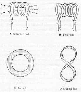
Fig. 14.3 Coils used to
emit fields and potentials.
A A standard coil emits
electric and magnetic fields in the space around it.
B In the bifilar
coil the electric and magnetic fields are cancelled, and electric scalar and
magnetic vector waves are produced.
C The torroidal
coil has the same effect.
D The Möbius coil produces only scalar waves.
The
information on coil properties is from Abraham (1998)
Due to (11)/(8) there is a lot of
possibilities to construct null-potential waves:
Example
Let U = f(k·x – ct) where f
is an arbitrary function and k be a unit vector. This generates the
potentials
φ = – μUt= μ c f ', A = grad U = k f ',
but, of course, the
physical quantities H,E,j, ρ generated by this null potential couple using the
representation formulas (1)-(4) vanish identically, i.e. the null-potential wave has no physical effect: It doesn’t
appear on the physical screen.
In contrast to the former result J. L. Oschman claims the
Aharonov-Bohm effect (AB-effect) to prove the meaning of a vector potential in
the physical world. The reader is referred to the literature for details, e.g.
http://www2.mathematik.tu-darmstadt.de/~bruhn/Aharonov.htm
We shall check this claim:
The AB-effect occurs
in the neighbourhood of a magnetic vector field H generated by a vector
potential A,
(1) H = curl A .
Evidently the effect depends on
the vector potential A, since its value is given by the boundary
integral
(12) ∫∂Ω A·dx
around the boundary ∂Ω of a check surface Ω, strangely enough, even when there was no magnetic field H at all along the path ∂Ω of integration (which can be realized by suited experimental configuration).
Indeed the AB-effect described by (12) attracted great
attention in the year of its discovery – until people realized that by applying
the well-known Stokes’ integral theorem to equation (12) it could be
transformed to
(13)
∫∂Ω A·dx = ∫∫Ω curl A ·do= ∫∫Ω H ·do.
But this result means that the AB-effect is calculable by
merely knowing the magnetic field H (on
the check surface Ω) without taking
into account any further "super world properties" of the potential A that are not already contained in the trace H = curl A.
The AB-effect does
not depend on "super world" properties of A that are not visible in the
physical world – the knowledge of H (on the "physical screen") is sufficient.
We can demonstrate this easily too by means of a null-potential wave, especially by means of its null-vector potential, which due to (11) has the form A0 = grad U: Hence the calculation of the AB-Effect of A0 using (12) yields
(14)
∫∂Ω A0·dx = ∫∂Ω grad U · dx = U(P) – U(P) = 0 ,
if we start the integration at an arbitrary point P of the boundary ∂ Ω and after one cycle of integration along ∂ Ω we stop the integration at P again.
This result (14) shows that the special information contained in a
null-vector potential A0 = grad U is just ignored by the AB-effect. Hence the
AB-effect doesn’t prove the physical meaning of a vector potential A for the physical world, since its
possible part A0 = grad U, which exceeds the
information contained in curl A, is always mapped to 0,
whatsoever the actual meaning of the
function U should be.
J.L. Oschman gives some further
statements on his "scalar waves", our
null-potential waves:
Scalar waves
appear to interact with atomic nuclei, rather than with electrons. Such
interactions are described by quantum chromodynamics (Ynduráin 1983).
We doubt that. Schrödinger’s
equation and other equations of atomic physics contain scalar potentials V. So
at first glance one might believe that here we would have a direct effect of
potential on the "physical screen". But the next glance shows that the potential
V is restricted by the condition V = 0 at infinity. This means that the
additional constant contained in V is fixed, and the information in V is
equivalent to that one in grad V, which is a force and hence a quantity of the
"physical screen". Therefore we guess that Oschman’s reference might be an
over-interpretation or misunderstanding of sources in physical literature.
The waves are
not blocked by Faraday cages or other kinds of shielding,
This statement could possibly be fulfilled by choice of the generating
function U. But it is physically worthless, since null-potential waves have –
as far as we know up to now – no physical effect, no traces on the "physical
screen".
they are
probably emitted by living systems, and they appear to be intimately involved
in healing (see e.g. Jacobs 1997, Rein 1998).
The sources given by J. L. Oschman seem not to be of physical
competency.
The scalar
potential has a peculiarity: it propagates instantaneously everywhere in space,
undiminished by distance.
This property of instantaneous propagation is what null-potential waves
can have by no means. Since they are generated by solutions U of the wave
equation (8) and are consequently solutions of the wave equations likewise. But
according to the theory of partial differential equations the wave equation
does not admit superluminal solutions.
Oschman’s "scalar waves" cannot
propagate with superluminal velocity.
At the end it could be of interest to compare Oschman’s concepts with
other concepts in literature: Ochman’s scalar wave is a potential (like
voltage) or a vector potential, while Meyl’s and Bearden’s scalar waves are
waves of electric or magnetic field vectors. There is no synthesis possible due
to its different units of measurement.
J.L. Oschman’s "scalar wave" concept is not compatible with the "scalar
waves" invented by T. Bearden or K. Meyl.
References
Abraham
G 1998 Potential shields against electromagnetic pollution: Synchroton Scalar
Synchronizer. Optimox Corporation, PO Box 3378, Torrance, CA 90510-3378.Tet:
800-U3-1601
Afilani
T L 1998 Device and method using dielectrokinesis to locate entities. US Patent
5,748,088
Ynduráin FJ
1983: Quantum chromodynamics: An Introduction ... Springer-Verlag
Appendix A: Potential representations of the fields of Electrodynamics
Under the assumption of constant material coefficients the
electrical charge density ρ(x,t), the current density j(x,t), the electric field
vector E(x,t) and the magnetic field vector H(x,t)
have to fulfil the "inhomogeneous" Maxwell-equations
(A1) curl E = – μ Ht ,
(A2) curl H = ε Et + j ,
(A3) ε div E = ρ ,
(A4) div H = 0 .
(A4) yields the existence of a vector potential A such that:
(A5) H
= curl A .
Inserting this into (A1) gives
(A6) curl (E
+ μ At) = 0
,
which proves the existence of a
(local) potentials φ such that
(A7)
E = – grad φ – μ At.
In order to fulfil (A2) also we
have to assume a relation between the potentials φ, A.
>From (A2) we obtain by using (A5) and (A7):
j
= curl H – ε Et
(A8)
= curl curl A – ε (–μ Att – grad φ)
= grad (div A + ε φt) – (ΔA – 1/c²
Att) .
If we couple the potentials φ, A by the Lorenz-condition (falsely ascribed to due to H.A. Lorentz)
(A9) div A + ε φt = 0
(which means that we prescribe the sources of A in addition to prescribing its curl
by (A5), which is permissible therefore), we obtain the vector potential
representation of the current density
(A10) j = 1/c² Att – Δ
A .
Similarly (A3) and (A9) yield the potential
representation of the charge distribution ρ:
(A11) ρ = ε div E = ε (1/c² φtt –
Δφ).
Altogether taking (A5) = (1), (A7)
= (2), (A10) = (3) and (A11) = (4) we have the desired potential representations of the physical field quantities E, H, j
and ρ.
Appendix B: Null-Potential-Waves ("Scalar Waves")
Null-potential waves, J. L.
Oschman’s "scalar
waves", are defined as potential
couples (φ0,A0), the generated physical fields of
which are completely cancelled by destructive interference. Hence we have
(B1) H0 = curl A0 = 0 ,
(B2) E0 = – grad φ0 – μ A0 t = 0 ,
(B3)
j0 = 1/c² A0 tt – Δ
A0 = 0 ,
(B4)
ρ0 = 1/c² φ0 tt – Δ φ0 = 0 .
Additionally we have to fulfil the Lorenz-condition (falsely ascribed to due to H.A. Lorentz)
(B5) div A0 + ε φ0 t = 0 .
(B1) implies
(B6)
A0 =
grad V
where V is some scalar function.
Then (B2) yields
grad (φ0 + μ Vt) = 0 ,
hence
(B7)
φ0 = – μ (Vt + χ·(t))
with some function χ(t).
But due to grad U = grad V for U = V + χ we obtain
(B6') A0 = grad U
and
(B7') φ0 = – μ Ut
Using the Lorenz-condition (falsely ascribed to due to H.A. Lorentz) (B5) yields the necessary condition for U, the wave equation:
(B8) 1/c² Utt – Δ U = 0 .
Conversely (B8) is sufficient to establish the
representations (B1)-(B4) by using (B6') and (B7'):
The solutions U
of the wave equation (and these only)
generate null-potential waves.
The wave equation is one of the best-known equations in the
Theory of Partial Differential Equations. An important theorem says that signal
propagation cannot exceed the speed of light c.
The wave equation
has no superluminal solutions, hence no superluminal
null-potential
waves are possible.
Remark on the Lorenz-Condition falsely ascribed to H.A. Lorentz
The Lorenz condition stems from
Lorenz, L. "On the Identity of the Vibrations of Light with Electrical Currents." Philos. Mag. 34, 287-301, 1867.
Further References
van Bladel, J. "Lorenz or Lorentz?" IEEE Antennas Prop. Mag. 33, 69, 1991.
Whittaker, E. A History of the Theories of Aether and Electricity, Vols. 1-2. New York: Dover, p. 268, 1989.