30 May 2008
This is a comment (in blue) on the math contained in Meyl's papers which is quoted here in
black in parts. There are a lot of dubious and wrong verbal formulations in and between the lines which I don't comment on. Meyl's ''math'' is sufficiently convincing also without taking the verbal text into consideration.There are two almost independent attempts by Meyl to prove the existence of ''scalar waves'' which denotation is used by Meyl as synonymous with ''longitudinal em waves'':
1. Meyl's ''new and dual field approach''.
2. Meyl's ''fundamental field equation''.
Both attempts go astray as will be shown below.
In
Sect. 1.4, eqs. (1.1-11), assuming a linear Ohm law (1.5), Meyl derives a damped wave
equation (1.11) for the field vector E, asking for ''longitudinal wave
components hidden'' in eq. (1.11).
His supposition is missing ''duality'' of the eqs. (1.1-11) and especially
eq. (1.14),
and therefore long verbose passages follow (Sects. 1.6-7 and 2.1-9) to prepare
Meyl's idea
of a ''new and dual field approach'' given according to Meyl by the
eqs (2.1) and (2.3).
These equations are taken from W.R. Pohl's book [14] where an em wave
is considered that passes along as a whole at constant velocity u watched by an observer at rest.
(Meyl uses −v instead of u.)
Seemingly Meyl does not recognize that this is a very special wave: Pohl remarks that this wave
is transversal wave travelling at speed of light c. Therefore Pohl's waves
are not at all a well-suited basis for someone who is attempting to develop a theory
of longitudinal em waves.
Meyl, ignoring these shortcomings of his ''new approach'', nevertheless attempts to
derive a
new wave equation (4.9), ignoring that his Pohl waves in case of
ρel = div D ≠ 0
and/or ρmg = div B ≠ 0 would be accompanied by
(electric or magnetic) charge transports at speed of light
in direction of the wave propagation −v.
Even if one accepts this hypothesis of charges moving at c, in addition Meyl assumes
that the
corresponding currents
jel = −v ρel
and
jmg = −v ρmg
are subject to linear Ohm's laws
jel = σelE
and
jmg = σmgH
respectively. This implies
E | | v
and
H | | v
in contradiction to the transversality of E and H according to Meyl's
basic eqs. (2.1) and (2.3).
Meyl does not at all fear contradicting himself, if the statements have some verbal distance at least:
In
Sect 5.4 he gives pictures of magnetic and electric ring vortices
that are allegedly due to N. Tesla (as communicated by Meyl).
Evidently each figure is contradicting the
transversality of both the magnetic and the electric field as implied by his
equations of ''new approach'' and assured by
R.W. Pohl.
Apparently Meyl erroneously believes that
only one of the
two Pohl equations must be fulfilled in each case.
Due to these inconsistencies (and additional math errors) Meyl's ''new and dual field approach''
fails.
There is a part in Meyl's developments that might be considered independently
of the inconsistency of the ''new approach'':
The calculations of
Sect.4.1, the eqs. (4.1-5) which yield the ''fundamental
field equation'' (4.5) (FFE). If there exist Meyl's scalar waves (longitudinal waves) within the
scope of the eqs. (4.1-5) then these waves should satisfy the FFE.
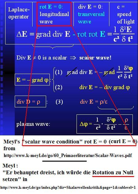
What is a scalar wave, say E? A field that can be derived from a scalar potential
Φ, E = grad Φ, which is locally equivalent with the scalar wave condition
curl E = 0 .
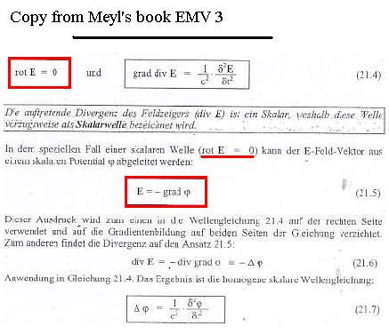
In the past, Meyl agreed with that condition (see e.g. his book
EMV3 or p.201 of his paper
Scalar Waves: Theory and Experiments,
Journal of Scientific Exploration, Vol. 15, No. 2, pp. 199–205, 2001).
However, in the meantime he learned that curl E = 0 would be disastrous
for his scalar wave claim (see Remark 3.3) and so
he denies all. To sum up,
Meyl's papers under review here are completely wrong and useless, written by
someone who lacks any deeper understanding of the topics he is dealing with.
Pohl's Waves suited for Meyl's ''NewApproach''?
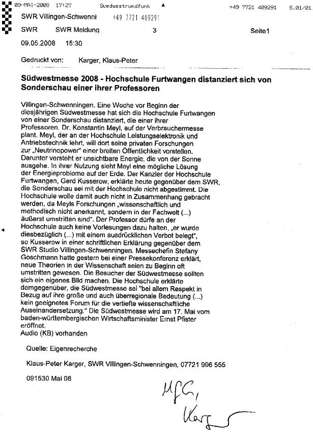
SW-Messe2008: Hochschule Furtwangen distanziert sich von Prof. Meyls Sonderschau1. The ''new and dual field approach''
2. The ''fundamental field equation''
Introduction summary
→ Remark 1
Further links
ANNUAL 2006 OF THE CROATIAN ACADEMY OF ENGINEERING
Proceedings of the 1st RFID Eurasia Conference Istanbul 2007, IEEE Catalog Number: 07EX1725, page 78-89
by Prof. Konstantin Meyl, Ph.D.
Faculty of Computer and Electrical Engineering
Furtwangen University, Germany
A short derivation brings it to light. We start with the law of induction according to the textbooks
curl E = – δB/δt (1.1)
with the electric field strength E = E(r,t) and the magnetic field strength H = H(r,t) and:
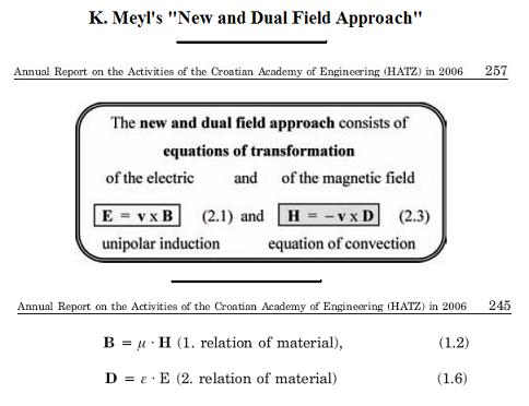
B = μ · H (1. relation of material), (1.2)
apply the curl-operation to both sides of the equation
– curl curl E = μ · δ(curl H)/δt (1.3)
and insert in the place of curl H Ampčre’s law:
curl H = j + δD/δt (1.4)
with
j = σ · E (Ohm’s law) (1.5)
with
D = ε · E (2. relation of material) (1.6)
and
τ1 = ε/σ (relaxation time [5]) (1.7)
curl H = ε · (E/τ1 + δE/δt) (1.8)
– curl curl E = μ · ε · (1/τ1 · δE/δt + δ˛E/δt˛) (1.9)
with the abbreviation:
μ · ε = 1/c˛. (1.10)
The generally known result describes a damped electro-magnetic wave [6]:
– curl curl E · c˛ = δ˛E/δt˛ + (1/τ1) · δE/δt
(1.11)
transverse – wave + vortex damping
On the one hand it is a transverse wave. On the other hand there is an damping term in the equation, which is responsible for the losses of an antenna. It indicates the wave component, which is converted into standing waves, which can be also called field vortices, that produce vortex losses for their part with the time constant τ1 in the form of heat.
Where however do, at close range of an antenna proven and with transponders technically used longitudinal wave components hide themselves in the field equation (1.11)?
The wave equation found in most textbooks has the form of an inhomogeneous Laplace equation. The famous French mathematician Laplace considerably earlier than Maxwell did find a comprehensive formulation of waves and formulated it mathematically:
Δ E · c˛ = – curl curl E · c˛ + grad div E · c˛ = δ˛E/δt˛ (1.12)
Laplace transverse
- longitudinal - wave
operator (radio wave) (scalar wave)
On the one side of the wave equation the Laplace operator stands, which describes the spatial field distribution and which according to the rules of vector analysis can be decomposed into two parts. On the other side the description of the time dependency of the wave can be found as an inhomogeneous term.
If the wave equation according to Laplace (1.12) is compared to the one, which the Maxwell equations have brought us (1.11), then two differences clearly come forward:
1. In the Laplace equation the damping term is missing.
2. With divergence E a scalar factor appears in the wave equation, which founds a scalar wave.
One practical example of a scalar wave is the plasma wave. This case forms according to the
3. Maxwell equation:
div D = ε · div E = ρel (1.13)
the space charge density consisting of charge carriers ρel the scalar portion. These move in form of a shock wave longitudinal forward and present in its whole an electric current.
Since both descriptions of waves possess equal validity, we are entitled in the sense of a coefficient comparison to equate the damping term due to eddy currents according to Maxwell (1.11) with the scalar wave term according to Laplace (1.12).
Physically seen the generated field vortices form and establish a scalar wave.
The presence of div E proves a necessary condition for the occurrence of eddy currents. Because of the well known skin effect [7] expanding and damping acting eddy currents, which appear as consequence of a current density j , set ahead however an electrical conductivity 1 (acc. to eq. 1.5).
Within the near field range of an antenna opposite conditions are present.
With bad conductivity in a general manner a vortex with dual characteristics
would be demanded for the formation of longitudinal wave
components. I want to call this contracting antivortex, unlike to the expanding
eddy current, a potential vortex.
If we examine the potential vortex with the Maxwell equations for validity
and compatibility, then we would be forced to let it fall directly again.
The derivation of the damped wave equation (1.1 to 1.11) can take place
in place of the electrical, also for the magnetic field strength. Both wave
equations (1.11 and 1.12) do not change thereby their shape. In the
inhomogeneous Laplace equation in this dual case however, the longitudinal
scalar wave component through div H is described and this is according
to Maxwell zero!
4. Maxwell’s equation:
div B = μ · div H = 0
(1.14)
If is correct, then there may not be a near field, no wireless transfer of
energy and finally also no transponder technology. Therefore, the correctness
is permitted (of eq. 1.14) to question and examine once, what would
result thereby if potential vortices exist and develop in the air around an
antenna scalar waves, as the field vortices form among themselves a
shock wave.
Besides still another boundary problem will be solved: since in div D electrical
monopoles can be seen (1.13) there should result from duality to
div B magnetic monopoles (1.14). But the search was so far unsuccessful
[8]. Vortex physics will ready have an answer.
If a measurable phenomenon should, e.g. the close range of an antenna,
not be described with the field equations according to Maxwell mathematically,
then prospect is to be held after a new approach. All efforts
that want to prove the correctness of the Maxwell theory with the
Maxwell theory end inevitably in a tail-chase, which does not prove anything
in the end.
In a new approach high requirements are posed. It may not contradict
the Maxwell theory, since these supply correct results in most practical
cases and may be seen as confirmed. It would be only an extension permissible,
in which the past theory is contained as a subset e.g. Let’s go on
the quest.
If the by Bosse [13] prompted term “equation of transformation” is justified
or not at first is unimportant. That is a matter of discussion.
If there should be talk about equations of transformation, then the dual
formulation (to equation 2.1) belongs to it, then it concerns a pair of
equations, which describes the relations between the electric and the
magnetic field.
The new and dual field approach consists of
2. The approach
2.1 Faraday instead of Maxwell
2.2 Vortex and anti-vortex
. . . . . . . . . . . . . . . . . .
2.3 The Maxwell approximation
. . . . . . . . . . . . . . . . . .
2.4 The mistake of the magnetic monopole
. . . . . . . . . . . . . . . . . .
2.5 The discovery of the law of induction
. . . . . . . . . . . . . . . . . .
2.6 The unipolar generator
. . . . . . . . . . . . . . . . . .
2.7 Different induction laws
. . . . . . . . . . . . . . . . . .
2.8 The electromagnetic field
. . . . . . . . . . . . . . . . . .
2.9 Contradictory opinions in textbooks
. . . . . . . . . . . . . . . . . .
2.10 The equation of convection
equations of transformation
E = v × B
(2.1)
and
H = − v × D
(2.3)
unipolar induction
equation of convection
Written down according to the rules of duality there results an equation (2.3), which occasionally is mentioned in some textbooks. While both equations in the books of Pohl [14, p.76 and 130] and of Simonyi [15] are written down side by side having equal rights and are compared with each other, Grimsehl [16] derives the dual regularity (2.3) with the help of the example of a thin, positively charged and rotating metal ring. He speaks of “equation of convection”, according to which moving charges produce a magnetic field and so-called convection currents. Doing so he refers to workings of Röntgen 1885, Himstedt, Rowland 1876, Eichenwald and many others more, which today hardly are known.
In his textbook also Pohl gives practical examples for both equations of
transformation. He points out that one equation changes into the other
one, if as a relative velocity v the speed of light c should occur.
Not at
[11, p.130]. Where?
As repeatedly criticized in the past, see e.g. p.11 of
http://www2.mathematik.tu-darmstadt.de/~bruhn/EMV3-Kritik.doc
it will be pointed out here again Meyl's ''new and dual field approach''
is a flop.
Pointing to K. Simonyi [15, p.498] is at least misleading. Simonyi's equations
E' = E + v × B and H' = H − v × D
are indeed ''transformation equations'' between a frame S at rest and a frame S' moving relative to S at velocity v where the nonrelativistic case |v| << c is assumed. However, Meyl doesn't use these equations.
Meyl takes his basic ''equations of transformation''
E = v × B and H = − v × D .
originally from
R.W. Pohl's book [11] (v = −u)
where |v| = |u| = c is assumed,
but seemingly not realized by Meyl. Pohl's equations describe the case of an em wave
that is moving with constant velocity u = −v.
Pohl points out on p.130 that the field (E,H) is travelling
at velocity c in direction of u and the vectors E, H, u
must be pairwise perpendicular, in other words, a transversal em wave.
But now there is no transformation: The denotation ''Equations of transformation''
is completely inappropriate and misleading.
First conclusions from
Meyl's basic equations (2.1) and (2.3)
are the transversality relations to be obtained
from the elementary rules of vector algebra
v ^ E ^
H ^ v ,
together with the velocity condition
εμ v˛ = 1 ,
thus
|v| = c = 1/(εμ)½
to be obtained by inserting one of
Meyl's basic equations (2.1) and (2.3)
into the other one using the well-known vector identity
v ×(v × a) = (v · a) v −
(v · v) a
where
a = εμ E
or
a = εμ H .
The results, orthogonality relations and velocity condition are explicitely mentioned by R.W. Pohl at
[1, p.130].
Let i, j, k be the pairwise perpendicular Cartesian unit vectors
of a (x,y,z)-coodinate frame, v± = ± c k and Ao some constant > 0.
Then from (MFE) we obtain the vector fields
H± = Ao eiω(t±z/c) i,
B± = μ H± = μ Ao eiω(t±z/c) i,
E± = v± × B = ± c μ Ao eiω(t±z/c) j,
D±
= ε E±
= c εμ Ao eiω(t±z/c) j
and finally
− v± × D± = − c˛ εμ k ×
Ao eiω(t±z/c) j =
c i Ao eiω(t±z/c) = H±
Hence for each sign + or − separately
Meyl's basic equations are fulfilled
by the fields H±, B±, E± and D±,
as can easily checked by the reader.
These fields constitute two counter-running plane waves which therefore satisfy
the homogeneous Maxwell equations, and, consequently, the sums
H++H−, B++B−,
E++E− and D++D−
as well. However, these sums do not satisfy Meyl's basic eqs. since an appropriate multiplicator
v (with |v|=c) cannot be found:
1.2 The velocity v
In general, these orthogonality relations are not fulfilled
by the solutions of the Maxwell equations.1.3 Superposition of waves?
Meyl's basic eqs. do not fulfil the superposition principle of waves,
which is satisfied by the homogeneous Maxwell equations.
→ Remark 2
We now have found a field-theoretical approach with the equations of transformation, which in its dual formulation is clearly distinguished from the Maxwell approach. The reassuring conclusion is added: The new field approach roots entirely in textbook physics, as are the results from the literature research. We can completely do without postulates. Next thing to do is to test the approach strictly mathematical for freedom of contradictions. It in particular concerns the question, which known regularities can be derived under which conditions. Moreover the conditions and the scopes of the derived theories should result correctly, e.g. of what the Maxwell approximation consists and why the Maxwell equations describe only a special case.
As a starting-point and as approach serve the equations of transformation of the electromagnetic field, the Faraday-law of unipolar induction (2.1) and the according to the rules of duality formulated law called equation of convection (2.3).
E = v × B (2.1)
and
H = − v × D (2.3)
If we apply the curl to both sides of the equations:
curl E = curl (v × B) (3.1)
and
curl H = − curl (v × D) (3.2)
then according to known algorithms of vector analysis the curl of the cross product each time delivers the sum of four single terms [17]:
curl E = (B grad)v − (v grad)B + v div B − B div v (3.3)
curl H = −[(D grad)v − (v grad)D + v div D − D div v] (3.4)
Two of these again are zero for a non-accelerated relative motion in the x-direction with:
v = dr/dt (3.5)
grad v = 0 (3.5*)
and
div v = 0 . (3.5**)
One term concerns the vector gradient (v grad)B, which can be represented
as a tensor. By writing down and solving the accompanying derivative
matrix giving consideration to the above determination of the v-vector,
the vector gradient becomes the simple time derivation of the field
vector B(r(t)),
(v grad)B = dB/dt
and
(v grad)D = dD/dt ,
(3.6)
according to the rule [17]:
dV(r(t))/dt = ∂V(r=r(t))/∂r · dr(t)/dt = (v grad)V. (3.7)
The vector fields under consideration are depending on the spatial vector r and time t in four-dimensional spacetime, e.g. written after eq. (1.1) as E = E(r,t) and H = H(r,t), fitting for the application of the spatial partial differential operators div, grad and curl, and the partial time-differential-operator ∂/∂t, the differential operators of the Maxwell equations.
However, starting with his eq. (2.1), Meyl changes the concept: Instead of correctly assuming E = E(r,t) he now writes E = E(r(t)), analogously for the other fields. This is a misinterpretation of Pohl's wave condition that the complete em wave (E,H) should travel along at constant velocity u = −v in Pohl's book): Meant is the special dependency E = E(r−ut) and H = H(r−ut). For that case the multi-dimensional chain rule has to be applied to a function F(x(r,t)) where x(r,t) = r−ut, yielding
∂F/∂t = [∂x(r,t)/∂t · gradx) F(x]|x=r−ut = −[u · gradx F(x)]|x=r−ut
i.e. in a somewhat simplified shorthand notation (suppressing the index x):
∂E/∂t = − u · grad E(x)|x=r−ut = v · grad E and ∂H/∂t = v · grad H (3.6')
It must be emphasized here again that the rules (3.6') are valid only for fields
depending on the special combination
r − ut = r + vt, the special
case of Meyl's ''new approach''but not for the general case.
Applications of the invalid eqs. (3.6) will be marked in red
in the sequel and supplemented by adding the correct relation in blue
numbered with the primed equation number.
.
2.2.1 Roughly spoken Meyl's chain rule error can be ''repaired'' by replacing
d/dt with ∂/∂t.
2.2.2 Concerning the subsequent settings (3.10) and (3.11) we should remember the condition
|v| = c that was found in Remark 1.1.
As a consequence of eq. (3.11) Meyl's
carriers of electrical charge, i.e. in traditional theory the electrons, must without exception move with speed of light.
And eq. (3.10) gives the same for the hypothetical magnetic monopoles, a very strange result
of Meyl's ''theory''. The invalid consequences are marked in
magenta.2.2 Further remarks
→ Remark 3
For the last not yet explained terms at first are written down the vectors
b and j as abbreviation.
curl E = − dB/dt + v div B = − dB/dt − b
(3.8)
curl E = − ∂B/∂t + v div B = − ∂B/∂t − b
(3.8')
curl H = dD/dt − v div D = dD/dt + j
(3.9)
curl H = ∂D/∂t − v div D =
∂D/∂t + j
(3.9')
With equation 3.9 we in this way immediately look at the well-known law of Ampčre (1st Maxwell equation).
The result will be the Maxwell equations, if:
• the potential density b = − v div B
= u div B = 0 ,
(3.10)
(eq. 3.8 ≡ law of induction 1.1, if b = 0 resp. div B = 0)!
• the current density j = − v div D =
= u ρel = − v · ρel ,
(3.11)
(eq. 3.9 ≡ Ampčre’s law 1.4, if j ≡ with v moving negative
(eq. 3.9 ≡ Ampčre’s law 1.4, if j ≡ with u = −v
moving
charge carriers, (ρel = electric space charge density).
The comparison of coefficients (3.11) in addition delivers a useful explanation to the question, what is meant by the current density j: it is a space charge density ρel consisting of negative charge carriers, which moves with the velocity v for instance through a conductor (in the x-direction). The current density j and the dual potential density b mathematically seen at first are nothing but alternative vectors for an abbreviated notation. While for the current density j the physical meaning already could be clarified from the comparison with the law of Ampčre, the interpretation of the potential density b still is due:
b = – v div B = u div B (= 0) , (3.10)
>From the comparison of eq. 3.8 with the law of induction (eq.1.1) we merely infer, that according to the Maxwell theory this term is assumed to be zero. But that is exactly the Maxwell approximation and the restriction with regard to the new and dual field approach, which roots in Faraday.
Assuming, a monopole concerns a special form of a field vortex, then immediately gets clear, why the search for magnetic poles has to be a dead end and their failure isn’t good for a counterargument: The missing electric conductivity in vacuum prevents current densities, eddy currents and the formation of magnetic monopoles. Potential densities and potential vortices however can occur. As a result can without exception only electrically charged particles be found in the vacuum.
Let us record: Maxwell’s field equations can directly be derived from the new dual field approach under a restrictive condition. Under this condition the two approaches are equivalent and with that also error free. Both follow the textbooks and can so to speak be the textbook opinion.
The restriction (b = 0) surely is meaningful and reasonable in all those cases in which the Maxwell theory is successful. It only has an effect in the domain of electrodynamics. Here usually a vector potential A is intro- duced and by means of the calculation of a complex dielectric constant a loss angle is determined. Mathematically the approach is correct and dielectric losses can be calculated. Physically however the result is extremely questionable, since as a consequence of a complex a complex speed of light would result, according to the definition:
c = 1/sqr(εμ) . (3.12)
With that electrodynamics offends against all specifications of the textbooks, according to which c is constant and not variable and less then ever complex. But if the result of the derivation physically is wrong, then something with the approach is wrong, then the fields in the dielectric perhaps have an entirely other nature, then dielectric losses perhaps are vortex losses of potential vortices falling apart?
Is the introduction of a vector potential A in electrodynamics a substitute
of neglecting the potential density b? Do here two ways mathematically
lead to the same result? And what about the physical relevance? After
classic electrodynamics being dependent on working with a complex constant
of material, in what is buried an insurmountable inner contradiction,
the question is asked for the freedom of contradictions of the new
approach. At this point the decision will be made, if physics has to make a
decision for the more efficient approach, as it always has done when a
change of paradigm had to be dealt with.
The abbreviations j and b are further transformed, at first the current
density in Ampčre’s law
j = – v · ρel = u ρel
(3.11)
as the movement of negative electric charges.
By means of Ohm’s law
j = σ E
(1.5)
and the relation of material
D = ε E (1.6)
the current density
j = D/τ1
(3.13)
also can be written down as dielectric displacement current with the characteristic relaxation time constant for the eddy currents
τ1 = ε/σ . (1.7)
In this representation of the law of Ampčre:
curl H = dD/dt + D/τ1 = ε · (dE/dt + E/τ1) (3.14)
curl H = ∂D/∂t + D/τ1 = ε · (∂E/∂t + E/τ1) (3.14')
clearly is brought to light, why the magnetic field is a vortex field, and howthe eddy currents produce heat losses depending on the specific electric conductivity 1. As one sees we, with regard to the magnetic field description, move around completely in the framework of textbook physics.
Let us now consider the dual conditions. The comparison of coefficients
looked at purely formal, results in a potential density
b = B/τ2
(3.15)
in duality to the current density j (eq. 3.13), which with the help of an appropriate time constant τ2 founds vortices of the electric field. I call these potential vortices.
curl E = – dB/dt – B/τ2 = – μ · (dH/dt + H/τ2) (3.16)
curl E = – ∂B/∂t – B/τ2 = – μ (∂H/∂t + H/τ2) (3.16')
In contrast to that the Maxwell theory requires an irrotationality of the electric field, which is expressed by taking the potential density b and the divergence B equal to zero. The time constant τ2 thereby tends towards infinity.
There isn’t a way past the potential vortices and the new dual approach,
1. as the new approach gets along without a postulate,as well as
2. consists of accepted physical laws,
3. why also all error free derivations are to be accepted,
4. no scientist can afford to already exclude a possibly relevant phenomenon in at the approach,
5. the Maxwell approximation for it’s negligibleness is to examine,
6. to which a potential density measuring instrument is necessary,which may not exist according to the Maxwell theory.
With such a tail-chase always incomplete theories could confirm themselves.
It has already been shown, as and under which conditions the wave equation from the Maxwell' field equations, limited to transverse wave-portions, is derived (chapter 1.4). Usually one proceeds from the general case of an electrical field strength E = E(r,t) and a magnetic field strength H = H(r,t). We want to follow this example [18], this time however without neglecting and under consideration of the potential vortex term.
The two equations of transformation and also the from that derived field equations (3.14 and 3.16) show the two sides of a medal, by mutually describing the relation between the electric and magnetic field strength:
curl H = ∂D/∂t + D/τ1 = ε · (∂E/∂t + E/τ1) (4.1)
curl E = – ∂B/∂t – B/τ2 = – μ · (∂H/∂t + H/τ2) (4.2)
We get on the track of the meaning of the “medal” itself, by inserting the dually formulated equations into each other. If the calculated H-field from one equation is inserted into the other equation then as a result a determining equation for the E-field remains. The same vice versa also functions to determine the H-field. Since the result formally is identical and merely the H-field vector appears at the place of the E-field vector and since it equally remains valid for the B-, the D-field and all other known field factors, the determining equation is more than only a calculation instruction. It reveals a fundamental physical principle. I call it the complete or the “fundamental field equation”. The derivation always is the same: If we again apply the curl operation to curl E (lawof induction 4.2) also the other side of the equation should be subjected to the curl:
– curl curl E = μ · ∂(curl H)/∂t + (μ/τ2) · (curl H) (4.3)
If for both terms curl H is expressed by Ampčre’s law 4.1, then in total four terms are formed:
– curl curl E = μ · ε · [∂˛E/∂t˛ + (1/τ1) · E/ t + (1/τ2) · ∂E/∂t + E/τ1τ2] (4.4)
With the definition for the speed of light c:
ε · μ = 1/c˛, (1.10)
the fundamental field equation reads:
– c˛ · curl curl E = ∂˛E/∂t˛ + (1/τ1) · ∂E/∂t + (1/τ2) · ∂E/∂t
+ E/τ1τ2
a b c d e
(4.5)
(electromagnetic wave) + eddy current + potential vortex + I/U
The four terms are: the wave equation (a-b) with the two damping terms, on the one hand the eddy currents (a-c) and on the other hand the potential vortices (a-d) and as the fourth term the Poisson equation (a-e), which is responsible for the spatial distribution of currents and potentials [21].
Not in a single textbook a mathematical linking of the Poisson equation with the wave equation can be found, as we here succeed in for the first time. It however is the prerequisite to be able to describe the conversion of an antenna current into electromagnetic waves near a transmitter and equally the inverse process, as it takes place at a receiver. Numerous model concepts, like they have been developed by HF- and EMC-technicians as a help, can be described mathematically correct by the physically founded field equation.
In addition further equations can be derived, for which this until now was supposed to be impossible, like for instance the Schrödinger equation (Term d and e). As diffusion equation it has the task to mathematically describe field vortices and their structures.
As a consequence of the Maxwell equations in general and specifically the eddy currents (a-c) not being able to form structures, every attempt has to fail, which wants to derive the Schrödinger equation from the Maxwell equations. The fundamental field equation however contains the newly discovered potential vortices, which owing to their concentration effect (in duality to the skin effect) form spherical structures, for which reason these occur as eigenvalues of the equation. For these eigenvalue-solutions numerous practical measurements are present, which confirm their correctness and with that have probative force with regard to the correctness of the new field approach and the fundamental field equation [21]. By means of the pure formulation in space and time and the interchangeability of the field pointers here a physical principle is described, which fulfills all requirements, which a world equation must meet.
The Maxwell equations are nothing but a special case, which can be derived. (if 1/τ2= 0). The new approach however, which among others bases on the Faraday-law, is universal and can’t be derived on its part. It describes a physical basic principle, the alternating of two dual experience or observation factors, their overlapping and mixing by continually mixing up cause and effect. It is a philosophic approach, free of materialistic or quantum physical concepts of any particles.
Maxwell on the other hand describes without exception the fields of charged particles, the electric field of resting and the magnetic field as a result of moving charges. The charge carriers are postulated for this purpose, so that their origin and their inner structure remain unsettled.
With the field-theoretical approach however the field is the cause for the particles and their measurable quantisation. The electric vortex field, at first source free, is itself forming its field sources in form of potential vortex structures. The formation of charge carriers in this way can be explained and proven mathematically, physically, graphically and experimentally understandable according to the model.
Let us first cast our eyes over the wave propagation.
The first wave description, model for the light theory of Maxwell, was the inhomogeneous Laplace equation (1.12):
Δ E · c˛ = d˛E/dt˛
Δ E · c˛ = ∂˛E/∂t˛
with
ΔE = grad div E – curl curl E (4.6)
There are asked some questions:
• Can also this mathematical wave description be derived from the new approach?
• Is it only a special case and how do the boundary conditions read?
• In this case how should it be interpreted physically?
• Are new properties present,which can lead to new technologies?
Starting-point is the fundamental field equation (4.5). We thereby should remember the interchangeability of the field pointers, that the equation doesn’t change its form, if it is derived for H, for B, for D or any other field factor instead of for the E-field pointer. This time we write it down for the magnetic induction and consider the special case B(r(t)) [acc. to 19]:
– c˛ · curl curl B =
d˛B/dt˛
+ 1/τ2 dB/dt
+ 1/τ1 dB/dt
+ B/τ1τ2
(4.7)
– c˛ · curl curl B =
∂˛B/∂t˛
+ 1/τ2 ∂B/∂t
+ 1/τ1 ∂B/∂t
+ B/τ1τ2
(4.7')
that we are located in a badly conducting medium, as is usual for the wave propagation in air. But with the electric conductivity σ also 1/τ1 = σ/ε tends towards zero (eq. 1.7). With that the eddy currents and their damping and other properties disappear from the field equation, what also makes sense.
There remains the potential vortex term (1/τ2) · dB/dt , which using the already introduced relations
1/τ2 dB/dt = v grad B/τ2 (3.6)
involved with an in x-direction propagating wave
(v = (vx, vy= 0, vz= 0))
can be transformed directly into:
(1/τ2) · dB/dt = – ||v||˛ · grad div B.
(4.8)
The divergence of a field vector (div B) mathematically seen is a scalar, for which reason this term as part of the wave equation founds so-called “scalar waves” and that means that potential vortices, as far as they exist, will appear as a scalar wave. To that extent the derivation prescribes the interpretation.
v˛ grad div B – c˛ curl curl B = d˛B/dt˛
(4.9)
longitudinal transverse wave
with v = arbitrary with c = const. velocity of
(scalar wave) (em. wave) propagation
Meyl considers his equ. (4.9) as a generalization of the wave equation (1.12), here rewritten for B instead of E and slightly adapted:
c˛ grad div B – c˛ curl curl B = ∂˛B/∂t˛ (1.12')
longitudinal transverse wave
(scalar wave) (radio wave)
Following this assignment then for a medium with source-free field B, div B = 0, we would obtain a purely transversal wave while reversely in case of curl B = 0 we would have a purely longitudinal wave. Then from (4.9) we would obtain transversal waves (div B = 0) with velocity c while longitudinal waves (curl B = 0) would travel with velocity v where possibly v ≠ c (Meyl).
Independently of that, equ. (4.9) cannot be derived due to a further formula-error in eq. (4.8), which should correctly read as follows
(1/τ2) ∂B/∂t = – v (v · grad) div B. (4.8')
Since eq. (4.9) failed to be valid we are led back to Meyl's ''fundamental field equation'' (4.5). This equation is independent of Meyl's missed ''new and dual field approach'' and more general. The question is whether there exist longitudinal solutions E of eq. (4.5).
Meyl's condition for longitudinal solutions (scalar waves) E (see his book EMV3 also) is
curl E = 0 .
Inserting that in eq. (4.5) yields
0 = ∂˛E/∂t˛ + (1/τ1) · ∂E/∂t + (1/τ2) · ∂E/∂t + E/τ1τ2 . (4.5')
This is an ordinary differential equation for each point x in space, the general solution of which can be displayed here
E(x,t) = E1(x) e−t/τ1 + E2(x) e−t/τ2 (τ1 ≠ τ2) (4.5'')
where the vector fields E1(x) and E2(x) can be prescribed arbitrarily.
So, whatever his scalar wave condition be now, the reader should notice that at least a plane longitudinal wave must fulfil the condition (4.5'): Thus, at least,
The simplified field equation (4.7) possesses thus the same force of expression as the general wave equation (4.9), on adjustment of the coordinate system at the speed vector (in x-direction).
The wave equation (4.9) can be divided into longitudinal and transverse wave parts, which however can propagate with different velocity.
Physically seen the vortices have particle nature as a consequence of their structure forming property. With that they carry momentum, which puts them in a position to form a longitudinal shock wave similar to a sound wave. If the propagation of the light one time takes place as a wave and another time as a particle, then this simply and solely is a consequence of the wave equation.
Light quanta should be interpreted as evidence for the existence of scalar waves. Here however also occurs the restriction that light always propagates with the speed of light. It concerns the special case v = c. With that the derived wave equation (4.9) changes into the inhomogeneous Laplace equation (4.6).
The electromagnetic wave in general is propagating with c. As a transverse wave the field vectors are standing perpendicular to the direction of propagation. The velocity of propagation therefore is decoupled and constant. Completely different is the case for the longitudinal wave. Here the propagation takes place in the direction of an oscillating field pointer, so that the phase velocity permanently is changing and merely an average group velocity can be given for the propagation. There exists no restriction for v and v = c only describes a special case.
It will be helpful to draw, for the results won on mathematical way, a graphical model.
In high-frequency technology is distinguished between the near-field and the far-field. Both have fundamentally other properties.
Heinrich Hertz did experiment in the short wave range at wavelengths of some meters. From today’s viewpoint his work would rather be assigned the far-field. As a professor in Karlsruhe he had shown that his, the electromagnetic, wave propagates like a light wave and can be refracted and reflected in the same way.
Heinrich Hertz: electromagnetic wave (transverse)
Figure 6. The planar electromagnetic wave in the far zone.
It is a transverse wave for which the field pointers of the electric and the magnetic field oscillate perpendicular to each other and both again perpendicular to the direction of propagation. Besides the propagation with the speed of light also is characteristic that there occurs no phase shift between E-field and H-field.
The electromagnetic wave in general is propagating with c. As a transverse wave the field vectors are standing perpendicular to the direction of propagation. The velocity of propagation therefore is decoupled and constant. Completely different is the case for the longitudinal wave. Here the propagation takes place in the direction of an oscillating field pointer, so that the phase velocity permanently is changing and merely an average group velocity can be given for the propagation. There exists no restriction for v and v = c only describes a special case.
It will be helpful to draw, for the results won on mathematical way, a graphical model.
In the proximity it looks completely different. The proximity concerns distances to the transmitter of less than the wavelength divided by 2π. Nikola Tesla has broadcasted in the range of long waves, around 100 Kilohertz, in which case the wavelength already is several kilometres. For the experiments concerning the resonance of the earth he has operated his transmitter in Colorado Springs at frequencies down to 6 Hertz. Doing so the whole earth moves into the proximity of his transmitter. We probably have to proceed from assumption that the Tesla radiation primarily concerns the proximity, which also is called the radiant range of the transmitting antenna.
For the approach of vortical and closed-loop field structures derivations for the near-field are known [4].
The calculation provides the result that in the proximity of the emitting antenna a phase shift exists between the pointers of the E- and the H-field. The antenna current and the H-field coupled with it lag the E-field of the oscillating dipole charges for 90°.
Figure 7. The fields of the oscillating dipole antenna
In the text books one finds the detachment of a wave from the dipole accordingly explained.
If we regard the structure of the outgoing fields, then we see field vortices, which run around one point, which we can call vortex centre. We continue to recognize in the picture, howthe generated field structures establish a shock wave, as one vortex knocks against the next [see Tesla: 1]. Thus a Hertzian dipole doesn’t emit Hertzian waves! An antenna as near-field without exception emits vortices, which only at the transition to the far-field unwind to electromagnetic waves.
At the receiver the conditions are reversed. Here the wave (a-b in eq. 4.5) is rolling up to a vortex (a-c-d), which usually is called and conceived as a “standing wave”. Only this field vortex causes an antenna current (a-e) in the rod, which the receiver afterwards amplifies and utilizes. The function mode of sending and receiving antennas with the puzzling near field characteristics explain themselves directly from the wave equation (4.5).
How could a useful vortex-model for the rolling up of waves to vortices look like?
We proceed from an electromagnetic wave, which does not propagate after the retractor procedure any longer straight-lined, but turns instead with the speed of light in circular motion. It also furthermore is transverse, because the field pointers of the E-field and the H-field oscillate perpendicular to c. By means of the orbit the speed of light c nowhas become the vortex velocity.
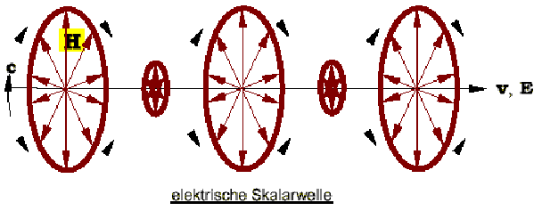
Nikola Tesla: electric scalar wave (longitudinal):
Wave and vortex turn out to be two possible and stable field configurations. For the transition from one into the other no energy is used; it only is a question of structure.
By the circumstance that the vortex direction of the ring-like vortex is determined and the field pointers further are standing perpendicular to it, as well as perpendicular to each other, there result two theoretical formation forms for the scalar wave. In the first case (fig. 9) the vector of the H-field points into the direction of the vortex centre and that of the E-field axially to the outside. The vortex however will propagate in this direction in space and appear as a scalar wave, so that the propagation of the wave takes place in the direction of the electric field. It may be called an electric wave.
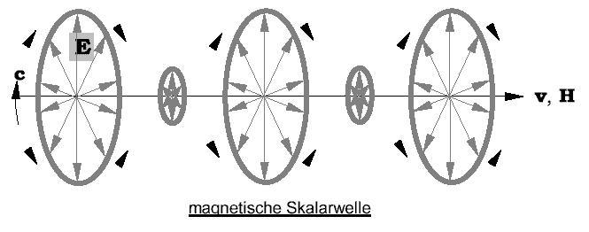
In the second case the field vectors exchange their place. The characteristic of the magnetic wave is that the direction of propagation coincides with the oscillating magnetic field pointer (fig.10), while the electric field pointer rolls up.
magnetic scalar wave (longitudinal):
Figure 9. Magnetic ring-vortices form an electric wave.
Figure 10. Electric ring-vortices form an magnetic wave.
The vortex picture of the rolled up wave already fits very well, because the propagation of a wave in the direction of its field pointer characterizes a longitudinal wave, because all measurement results are perfectly covered by the vortex model. In the text book of Zinke the near field is by the way computed, as exactly this structure is postulated! [20].
Longitudinal waves have, as well known, no firm propagation speed. Since they run toward an oscillating field pointer, also the speed vector v will oscillate. At so called relativistic speeds within the range of the speed of light the field vortices underlie the Lorentz contraction. This means, the faster the oscillating vortex is on it’s way, the smaller it becomes. The vortex constantly changes its diameter as a impulse-carrying mediator of a scalar wave.
Since it is to concern that vortices are rolled up waves, the vortex speed will still be c, with which the wave runs now around the vortex center in circular motion. Hence it follows that with smaller becoming diameter the wavelength of the vortex likewise decreases, while the natural frequency of the vortex increases accordingly.
If the vortex oscillates in the next instant back, the frequency decreases again. The vortex works as a frequency converter! The mixture of high frequency signals developed in this way distributed over a broad frequency band, is called noise.
Antenna losses concern the portion of radiated field vortices, which did not unroll themselves as waves, which are measured with the help of wide-band receivers as antenna noise and in the case of the vortex decay are responsible for heat development.
Spoken with the fundamental field equation (4.5) it concerns wave damping. The wave equation (4.9) explains besides, why a Hertz signal is to be only received, if it exceeds the scalar noise vortices in amplitude.
The proof could be furnished that within the Maxwell field equations an approximation lies buried and they only represent the special case of a new, dual formulated more universal approach. The mathematical derivations of the Maxwell field and the wave equation uncover, wherein the Maxwell approximation lies. The contracting antivortex dual to the expanding vortex current with its skin effect is neglected, which is called potential vortex. It is capable of a structural formation and spreads in badly conductive media as in air or in the vacuum as a scalar wave in longitudinal way.
At relativistic speeds the potential vortices underlie the Lorentz contraction. Since for scalar waves the propagation occurs longitudinally in the direction of an oscillating field pointer, the potential vortices experience a constant oscillation of size as a result of the oscillating propagation. If one understands the field vortex as an even however rolled up transverse wave, then thus size and wave-length oscillation at constant swirl velocity with c follows a continual change in frequency, which is measured as a noise signal. The noise proves as the potential vortex term neglected in the Maxwell equations. If e.g. with antennas a noise signal is measured, then this proves the existence of potential vortices. However if the range of validity of the Maxwell theory is left, misinterpretations and an excluding of appropriate phenomena from the field theory are the consequence, the noise or the near field cannot be computed any longer or conclusively explained.
If the antenna efficiency is very badly, for example with false adapted antennas, then the utilizable level sinks, while the antenna noise increases at the same time.
The wave equation following the explanation could also read differently: >From the radiated waves the transversals decrease debited to the longitudinal wave components. The latter’s are used however in the transponder technology as sources of energy, why unorthodox antenna structures make frequently better results possible, than usual or proven. Ball antennas proved in this connection as particularly favourable constructions. The more largely the ball is selected, the more can the reception range for energy beyond that of the near field be expanded. This effect can be validated in the experiment.
So far high frequency technicians were concerned only with the maximization of the transversal utilizable wave, so that this does not go down regarding the noise. The construction of far range transponders however require false adapted antennas, the exact opposite of what is learned and taught so far in the HF technology, inverse engineers and engineering so to speak. And in such a way the introduction and development of a new technology requires first an extended viewand neww ays of training.
1. N. Tesla, Art of transmitting electrical energy through the natural medium, United States Patent, No. 787,412 Apr. 1905
2. S. Kolnsberg, Drahtlose Signal- und Energieübertra-gung mit Hilfe von Hochfrequenztechnik in CMOS-Sensorsystemen (RFID-Technologie), Dissertation Uni Duisburg 2001.
3. Meinke, Gundlach: Taschenbuch der Hochfrequenztechnik, Springer Verl. 4.ed.1986, N2, eq.5
4. Zinke, Brunswig: Lehrbuch der Hochfrequenztechnik, 1. Band, Springer-Verlag, 3. ed. 1986, p. 335
5. G. Lehner, Elektromagnetische Feldtheorie, Springer Verlag 1990, 1st edition, page 239, aq. 4.23
6. K. Simonyi, Theoretische Elektrotechnik, vol. 20, VEB Verlag Berlin, 7th ed. 1979, page 654
7. K. Küpfmüller, Einführung in die theoretische Elektrotechnik, Springer Verl., 12th edit.1988, p.308
8. J.D. Jackson, Classical Electrodynamics. 2nd.ed. Wiley & Sons N.Y. 1975
9. H.J. Lugt, Wirbelströmung in Natur und Technik, G. Braun Verlag Karlsruhe 1979, table 21, p. 356
10. J.C. Maxwell, A treatise on Electricity and Magnetism, Dover Publications NewY ork, (orig. 1873).
11. R.W. Pohl, Einführung in die Physik, vol. 2 Elektrizitätslehre, 21.ed. Springer-Verlag 1975, pp. 76 and 130.
12. K. Küpfmüller, Einführung in die theoretische Elektrotechnik, Springer V. 12.ed.1988, p.228, eq.22.
13. G. Bosse, Grundlagen der Elektrotechnik II, BI-Hochschultaschenbücher No.183, 1. ed. 1967, Chapter 6.1 Induction, page 58
14. R.W. Pohl, Einführung in die Physik, vol. 2 Elektrizitätslehre, 21. ed. Springer-Verlag 1975, p. 77
15. K. Simonyi, Theoretische Elektrotechnik, vol. 20, VEB Verlag Berlin, 7.ed. 1979, page 924
16. Grimsehl: Lehrbuch der Physik, 2. vol., 17. ed. Teubner Verl. 1967, p. 130.
17. Bronstein et al: Taschenbuch der Mathematik, 4. Neuauflage Thun 1999, p. 652
18. G. Lehner, Elektromagnetische Feldtheorie, Springer Verlag 1990, 1.ed., p. 413 ff., chap. 7.1
19. J.C. Maxwell, A treatise on Electricity and Magnetism, Dover Publications N.Y., Vol. 2, pp. 438
20. Zinke, Brunswig: Lehrbuch der Hochfrequenztechnik, 1. vol., Springer-Verlag, 3. ed. 1986, p. 335
21. K. Meyl, Scalar Waves,from an extended vortex and field theory to a technical,bio - logical and historical use of longitudinal waves. Indel-Verlag (www.etzs.de) 1996, engl. Transl. 2003 Annual Report on the Activities of the Croatian Academy of Engineering (HATZ) in 2006 275
More than 100 Years ago Nikola Tesla has demonstrated three versions of transportation electrical energy:
1. the 3-phase-Network,as it is used today,
2. the one-wire-system with no losses and
3. the magnifying Transmitter for wireless supply.
The main subject of the conference presentation will be the wireless system and the practical use of it as a far range transponder (RFID for large distances). Let me explain some expressions as used in the paper. A “scalar wave” spreads like every wave directed, but it consists of physical particles or formations, which represent for their part scalar sizes. Therefore the name, which is avoided by some critics or is even disparaged, because of the apparent contradiction in the designation, which makes believe the wave is not directional, which does not apply however. The term “scalar wave” originates from mathematics and is as old as the wave equation itself, which again goes back on the mathematician Laplace. It can be used favourably as generic term for a large group of wave features, e.g. for acoustic waves, gravitational waves or plasma waves.
Seen from the physical characteristics they are longitudinal waves. Contrary to the transverse waves, for example the electromagnetic waves, scalar waves carry and transport energy and impulse. Thus one of the tasks of scalar wave transponders is fulfilled.
The term “transponder” consists of the terms transmitter and responder, describes thus radio devices which receive incoming signals, in order to redirect or answer to them. First there were only active transponders, which are dependent on a power supply from outside. For some time passive systems were developed in addition, whose receiver gets the necessary energy at the same time conveyed by the transmitter wirelessly.
![W.R. Pohl's book [14]](PohlS130.JPG)
![K. Simonyi [15, p.498]](SimonyiS924.JPG)